Example for analyzing flow on a planar surface#
The code below ascribes a flow to a planar disk-shaped surface and decomposes this flow into it’s curl-free and divergence-free components. If the user has gptoolbox installed, then we compare to Finite Element methods, but we simply skip this comparison if not.
%% DEC TEST FLAT CARTESIAN GEOMETRY =======================================
% This is a test of the Helmholtz-Hodge decomposition functionality of the
% Discrete Exterior Calculus implementation
%
% by Dillon Cislo and Noah P Mitchell 2022
%
%==========================================================================
clear; close all; clc;
%--------------------------------------------------------------------------
% Create a triangulation of the unit disk
%--------------------------------------------------------------------------
[tutorialDir, ~, ~] = fileparts(matlab.desktop.editor.getActiveFilename);
cd(tutorialDir)
load('testData.mat', 'diskTri')
cd('..')
% Re-create the triangulation
TR = diskTri ;
V = diskTri.Points ;
F = diskTri.ConnectivityList ;
% Edge connectivity list
E = edges(TR);
% Calculate centroid of faces
COM = cat( 3, V(F(:,1), :), V(F(:,2), :), V(F(:,3), :) );
COM = mean( COM, 3 );
% Calculate edge midpoints
Emp = ( V(E(:,2), :) + V(E(:,1),:) ) ./ 2;
%--------------------------------------------------------------------------
% Generate Discrete Exterior Calculus Object
%--------------------------------------------------------------------------
% profile on
DEC = DiscreteExteriorCalculus( F, V );
% profile viewer
%--------------------------------------------------------------------------
% View Results
%--------------------------------------------------------------------------
% triplot(TR);
% axis equal
%% ************************************************************************
% *************************************************************************
% COMPARE DEC DIFFERENTIAL OPERATORS TO FEM OPERATORS
% *************************************************************************
% *************************************************************************
clc;
%--------------------------------------------------------------------------
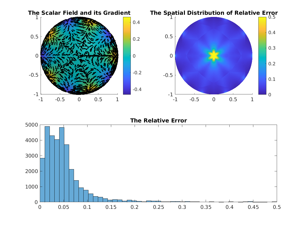
% Compare the Scalar Gradient Operator
%--------------------------------------------------------------------------
gradDEC = DEC.sharpPD * DEC.d0;
try
gradFEM = grad(V, F);
maxErr = max(abs(full(gradFEM(:)-gradDEC(:))));
fprintf('Maximum Difference in Gradient Operators = %f\n', maxErr);
catch
disp('To compare DEC against FEM results, install gptoolbox and add to your MATLAB path')
end
clear gradFEM gradDEC maxErr
%--------------------------------------------------------------------------
% Compare Scalar Laplacian Operator
%--------------------------------------------------------------------------
% The non-area weighted Laplacians
LN_DEC = DEC.dd1 * DEC.hd1 * DEC.d0;
try
LN_FEM = cotmatrix(V, F);
maxErr = max(abs(full(LN_FEM(:)-LN_DEC(:))));
fprintf('Maximum Difference in Bare Laplacian Operators = %f\n', maxErr);
clear LN_FEM LN_DEC
catch
disp('To compare DEC against FEM results, install gptoolbox and add to your MATLAB path')
end
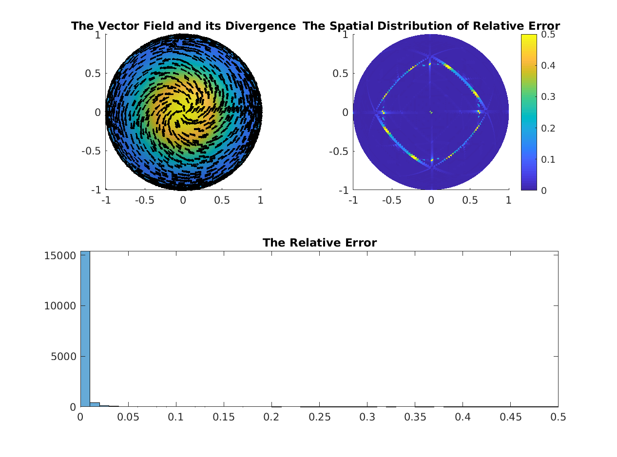
%--------------------------------------------------------------------------
% Compare Vector Divergence Operator
%--------------------------------------------------------------------------
divDEC = inv(DEC.hd0) * DEC.dd1 * DEC.hd1 * DEC.flatDP;
try
divFEM = div(V, F);
maxErr = max(abs(full(divFEM(:)-divDEC(:))));
fprintf('Maxumum Difference Between DEC Divergence and Bare FEM Divergence = %f\n', maxErr);
% Re-scale the bare FEM divergence operator
divFEM = 2 .* diag(invVA) * divFEM;
% THIS SCALING BRINGS THE ELEMENTS MUCH CLOSER TO EACH OTHER, BUT THEIR
% SPARSITY PATTERNS ARE DIFFERENT AND I DO NOT UNDERSTAND WHY
maxErr = max(abs(full(divFEM(:)-divDEC(:))));
fprintf('Maxumum Difference Between DEC Divergence and Weighted FEM Divergence = %f\n', maxErr);
clear divFEM divDEC maxErr
catch
disp('To compare DEC against FEM results, install gptoolbox and add to your MATLAB path')
end
%% ************************************************************************
% *************************************************************************
% TEST HELMHOLTZ-HODGE DECOMPOSITION
% *************************************************************************
% *************************************************************************
%--------------------------------------------------------------------------
% Design a tangent-vector field
%--------------------------------------------------------------------------
g = @(x,y) -exp( -(x.^2+y.^2) );
Ufunc = @(x,y) (-2 .* g(x,y)) .* [ (x-y), (x+y), zeros(size(x)) ];
U = Ufunc(COM(:,1), COM(:,2));
%--------------------------------------------------------------------------
% View Results
%--------------------------------------------------------------------------
% ssf = 20;
%
% triplot(triangulation(F, V(:, [1 2])));
% hold on
% quiver( COM(1:ssf:end,1), COM(1:ssf:end,2), ...
% U(1:ssf:end,1), U(1:ssf:end,2), ...
% 1, 'LineWidth', 2, 'Color', 'k' );
% hold off
% axis equal
%
% clear ssf
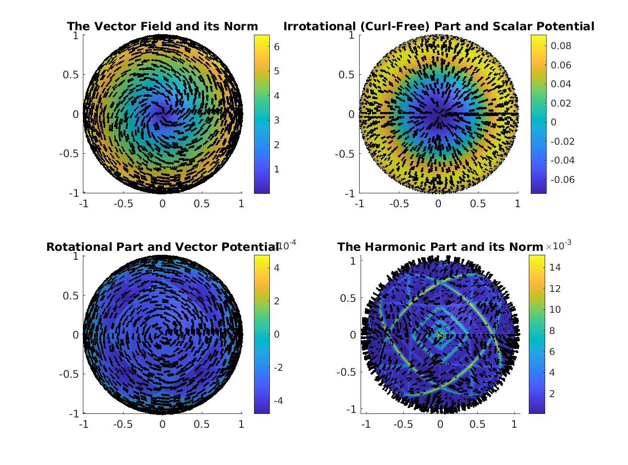
%% Perform Decomposition ==================================================
clc;
% Perform Helmholtz-Hodge decomposition
[divU, rotU, harmU, scalarP, vectorP] = ...
DEC.helmholtzHodgeDecomposition(U);
% Normalize rows for plotting
plotU = U ./ vecnorm(U, 2, 2);
plotDivU = divU ./ vecnorm(divU, 2, 2);
plotRotU = rotU ./ vecnorm(rotU, 2, 2);
plotHU = harmU ./ vecnorm(harmU, 2, 2);
% Sub-sampling factor for vector field visualization
ssf = 15;
figure
lw = 1 ; % line width for quiver arrows
% The full vector field ---------------------------------------------------
% Plot based on internal angles
s12 = vecnorm(V(F(:,2),:) - V(F(:,1),:), 2, 2);
s31 = vecnorm(V(F(:,3),:) - V(F(:,1),:), 2, 2);
s23 = vecnorm(V(F(:,3),:) - V(F(:,2),:), 2, 2);
a23 = acos((s12.^2 + s31.^2 - s23.^2)./(2.*s12.*s31));
a31 = acos((s23.^2 + s12.^2 - s31.^2)./(2.*s23.*s12));
a12 = acos((s31.^2 + s23.^2 - s12.^2)./(2.*s31.*s23));
internal_angles = [a23 a31 a12];
UColors = sparse( F(:), repmat(1:size(F,1),1,3), ...
internal_angles, size(V,1), size(F,1) );
UColors = UColors * U;
UColors = sqrt(sum(UColors.^2, 2));
subplot(2,2,1);
patch( 'Faces', F, 'Vertices', V, 'FaceVertexCData', UColors, ...
'FaceColor', 'interp', 'EdgeColor', 'none', ...
'SpecularStrength', 0.1, 'DiffuseStrength', 0.1, ...
'AmbientStrength', 0.8 );
hold on
quiver3( COM(1:ssf:end, 1), COM(1:ssf:end, 2), COM(1:ssf:end, 3), ...
plotU(1:ssf:end, 1), plotU(1:ssf:end, 2), plotU(1:ssf:end, 3), ...
1, 'LineWidth', lw, 'Color', 'k' );
hold off
axis equal tight
camlight
title('The Vector Field and its Norm');
colorbar
% The curl-free part ------------------------------------------------------
subplot(2,2,2);
patch( 'Faces', F, 'Vertices', V, 'FaceVertexCData', scalarP, ...
'FaceColor', 'interp', 'EdgeColor', 'none', ...
'SpecularStrength', 0.1, 'DiffuseStrength', 0.1, ...
'AmbientStrength', 0.8 );
hold on
quiver3( COM(1:ssf:end, 1), COM(1:ssf:end, 2), COM(1:ssf:end, 3), ...
plotDivU(1:ssf:end, 1), plotDivU(1:ssf:end, 2), plotDivU(1:ssf:end, 3), ...
1, 'LineWidth', lw, 'Color', 'k' );
hold off
axis equal tight
camlight
title('The Irrotational (Curl-Free) Part and the Scalar Potential');
colorbar
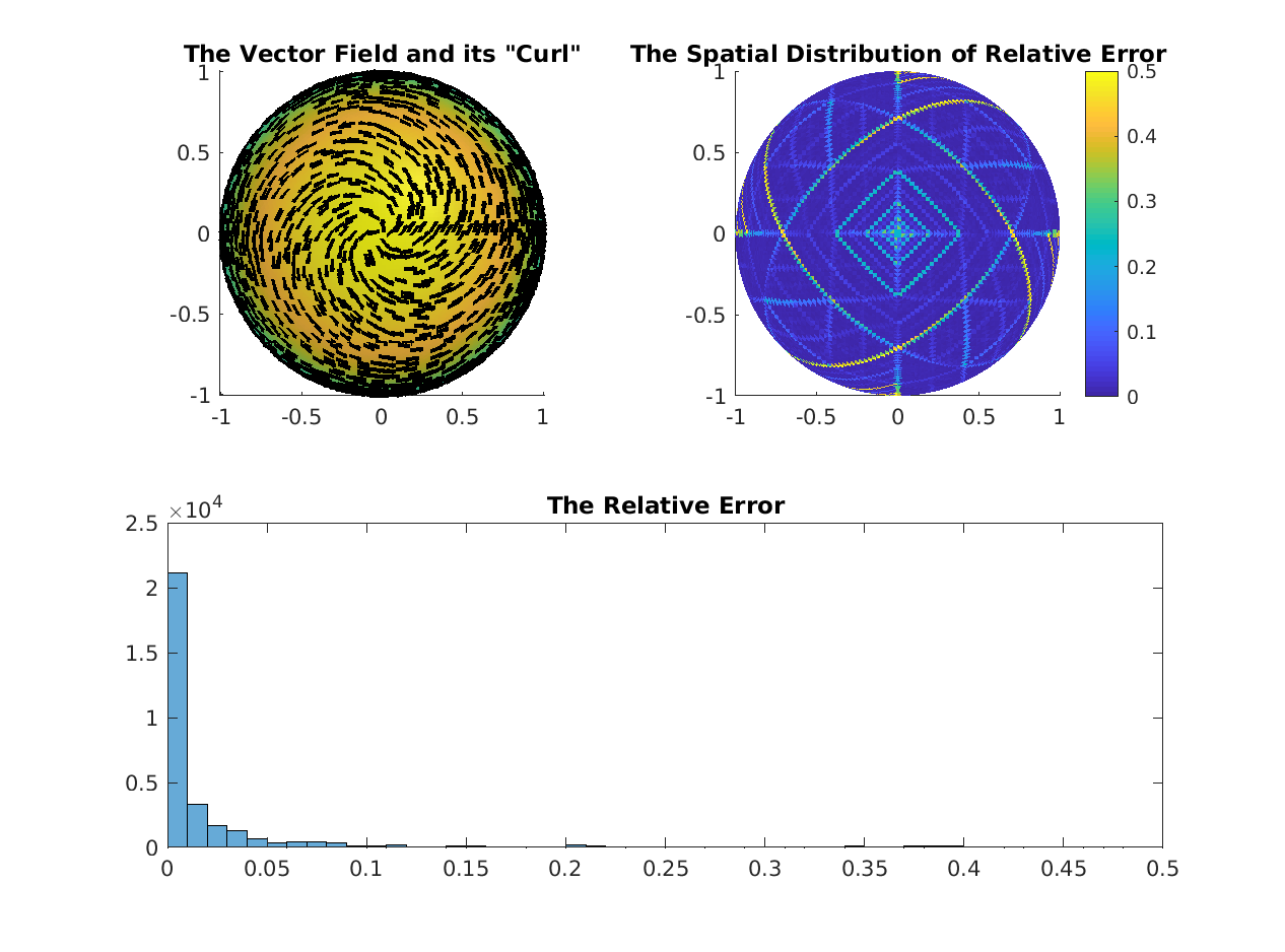
% The divergence-free part ------------------------------------------------
subplot(2,2,3);
patch( 'Faces', F, 'Vertices', V, 'FaceVertexCData', vectorP, ...
'FaceColor', 'flat', 'EdgeColor', 'none', ...
'SpecularStrength', 0.1, 'DiffuseStrength', 0.1, ...
'AmbientStrength', 0.8 );
hold on
quiver3( COM(1:ssf:end, 1), COM(1:ssf:end, 2), COM(1:ssf:end, 3), ...
plotRotU(1:ssf:end, 1), plotRotU(1:ssf:end, 2), plotRotU(1:ssf:end, 3), ...
1, 'LineWidth', lw, 'Color', 'k' );
hold off
axis equal tight
camlight
title('The Rotational (Divergence-Free) Part and the Vector Potential');
colorbar
% The harmonic part -------------------------------------------------------
HUColors = sparse( F(:), repmat(1:size(F,1),1,3), ...
internal_angles, size(V,1), size(F,1) );
HUColors = HUColors * harmU;
HUColors = sqrt(sum(HUColors.^2, 2));
subplot(2,2,4);
patch( 'Faces', F, 'Vertices', V, 'FaceVertexCData', HUColors, ...
'FaceColor', 'interp', 'EdgeColor', 'none', ...
'SpecularStrength', 0.1, 'DiffuseStrength', 0.1, ...
'AmbientStrength', 0.8 );
hold on
quiver3( COM(1:ssf:end, 1), COM(1:ssf:end, 2), COM(1:ssf:end, 3), ...
plotHU(1:ssf:end, 1), plotHU(1:ssf:end, 2), plotHU(1:ssf:end, 3), ...
1, 'LineWidth', lw, 'Color', 'k' );
hold off
axis equal tight
camlight
title('The Harmonic Part and its Norm');
colorbar
% clear ssf UColors HUColors plotU plotDivU plotRotU plotHU
%% CALCULATE ANALYIC RESULTS ==============================================
% NOTE: This section is only usable with the single supplied vector field.
% In principle one could solve the linear equations for the potentials
% analytically for an arbitrary vector field.
%
% The scalar and vector potentials are each only unique up to a pair of
% constants - their choice is arbitrary and can be absorbed into the
% harmonic component of the vector field. The discrete solution process
% will choose an unknown pair of constants to specify the potentials. In
% order to compare the solutions to analytic results we fit the constants
% to the numerical results in the least-squares sense
% Generate the scalar potential -------------------------------------------
A = [ log(sqrt(sum(V.^2, 2))), ones(size(V,1), 1) ];
A(isnan(A)) = 0; A(isinf(A)) = 0;
b = scalarP - g(V(:,1), V(:,2));
Cscalar = A \ b;
trueScalarP = g(V(:,1), V(:,2)) + Cscalar(2) + Cscalar(1) .* log(sqrt(sum(V.^2, 2)));
trueScalarP(isnan(trueScalarP)) = 0;
trueScalarP(isinf(trueScalarP)) = 0;
% Generate the vector potential -------------------------------------------
vectorP_OLD = vectorP;
vectorP = -full( DEC.hd2 * vectorP );
A = [ log(sqrt(sum(COM.^2, 2))), ones(size(COM,1), 1) ];
A(isnan(A)) = 0; A(isinf(A)) = 0;
b = vectorP - g(COM(:,1), COM (:,2));
Cvector = A \ b;
trueVectorP = g(COM(:,1), COM(:,2)) + Cvector(2) + Cvector(1) .* log(sqrt(sum(COM.^2, 2)));
trueVectorP(isnan(trueVectorP)) = 0;
trueVectorP(isinf(trueVectorP)) = 0;