Example for analyzing flow on a spherical surface#
The code below ascribes a flow to a spherical surface and decomposes this flow into it’s curl-free and divergence-free components. We also take a look at the Laplacian of the flow field on the surface and compare to analytic results (“ground truth”).
%% DEC Functionality Test =================================================
%
% This is a test of the functionality of the various methods of the
% 'Discrete Exterior Calculus' class.
%
% by Dillon Cislo and Noah P Mitchell 2022
%
%==========================================================================
clear; close all; clc;
%--------------------------------------------------------------------------
% Generate a surface triangulation
%--------------------------------------------------------------------------
% A triangulation of the unit sphere
[tutorialDir, ~, ~] = fileparts(matlab.desktop.editor.getActiveFilename);
cd(tutorialDir)
load('testData.mat', 'sphericalTri')
cd('..')
% Re-create the triangulation
TR = sphericalTri;
V = TR.Points;
F = TR.ConnectivityList;
% Edge connectivity list
E = edges(TR);
% Calculate centroid of faces
COM = cat( 3, V(F(:,1), :), V(F(:,2), :), V(F(:,3), :) );
COM = mean( COM, 3 );
% Calculate edge midpoints
Emp = ( V(E(:,2), :) + V(E(:,1),:) ) ./ 2;
%--------------------------------------------------------------------------
% Generate Discrete Exterior Calculus Object
%--------------------------------------------------------------------------
% profile on
DEC = DiscreteExteriorCalculus( F, V );
% profile viewer
disp('initiated DEC')
%--------------------------------------------------------------------------
% View Results
%--------------------------------------------------------------------------
% trisurf(TR);
% axis equal
%% ************************************************************************
% *************************************************************************
% GENERATE ANAYLTIC RESULTS FOR COMPARISON
% *************************************************************************
% *************************************************************************
syms theta phi x y z
assume( theta, 'real' ); assume( phi, 'real' );
assume( x, 'real'); assume( y, 'real'); assume( z, 'real' );
%==========================================================================
% Generate the Surface Parameters
%==========================================================================
% The equation of the surface
R = [ sin(theta) * cos(phi); sin(theta) * sin(phi); cos(theta) ];
% The tangent vectors
Etheta = [ gradient(R(1), theta); gradient(R(2), theta); gradient(R(3), theta) ];
Ephi = [ gradient(R(1), phi); gradient(R(2), phi); gradient(R(3), phi) ];
% The unit normal vector
% N = cross(Etheta, Ephi);
% N = simplify( N ./ sqrt( sum( N.^2 ) ) );
N = R;
% The metric tensor
g = simplify( [ dot(Etheta, Etheta), dot(Etheta, Ephi); ...
dot(Ephi, Etheta), dot(Ephi, Ephi) ] );
% The dual basis vectors
dtheta = Etheta;
dphi = Ephi ./ sin(theta).^2;
%==========================================================================
% Generate a Scalar Field on the Surface
%==========================================================================
%--------------------------------------------------------------------------
% Enter your favorite scalar field in Cartesian or spherical coordinates
% S = 1 / (1 + (x + 1/sqrt(2))^2 + z^2 ); DIVERGENT LAPLACIAN AT THETA = 0
S = (3/32) .* sqrt(77/pi) * sin(theta)^5 * cos(5*phi); % A spherical harmonic
%--------------------------------------------------------------------------
% Transform to spherical coordinates if necessary
S = simplify(subs( S, [x y z], [R(1) R(2) R(3)] ));
% Calculate the gradient of the scalar field
gradS = simplify( gradient(S, theta) * Etheta + ...
( gradient(S, phi) / sin(theta) ) * ( Ephi / sin(theta) ) );
% Calculate the Laplacian of the scalar field
lapS = simplify( ...
gradient( sin(theta) * gradient(S, theta), theta ) / sin(theta) + ...
gradient( gradient( S, phi ), phi ) / sin(theta)^2 );
%==========================================================================
% Generate a Vector Field on the Surface
%==========================================================================
%--------------------------------------------------------------------------
% Enter your favorite vector field in Cartesian or spherical coordinates
U = [ x * z * ( z^2 - 1/4 ) - y; ...
y * z * ( z^2 - 1/4 ) + x; ...
-( x^2 + y^2 ) * ( z^2 - 1/4 ) ];
%--------------------------------------------------------------------------
% Transform to spherical coordinates if necessary
U = simplify(subs( U, [x, y, z], [R(1) R(2) R(3)] ));
% Project onto the tangent space of the surface if necessary
U = U - dot(U, N) * N;
% Calculate the components of U in the (theta, phi)-basis
Utheta = simplify( dot(U, Etheta) / dot(Etheta, Etheta) );
Uphi = simplify( dot(U, Ephi) ./ dot(Ephi, Ephi) );
% Calculate the components of U in the dual basis
uTheta = Utheta;
uPhi = sin(theta)^2 * Uphi;
% Calculate the divergence of the vector field
divU = simplify( gradient( sin(theta) * uTheta, theta ) / sin(theta) + ...
gradient( uPhi, phi ) / sin(theta)^2 );
% Calculate the 'curl' of the vector field
% MIGHT NEED AN EXTRA-FACTOR OF THE AREA FORM
curlU = simplify(...
(gradient( uPhi, theta ) - gradient( uTheta, phi )) / sin(theta) );
% Calculate the Laplacian of the vector field
% IMPLEMENT THIS!!!!
%% Convert Symbolic Quantities to Numerical Quantities ====================
fprintf('Substituting numerical values for symbolic variables... ');
% (theta, phi) for each vertex
NTheta = acos(V(:,3));
NPhi = atan2(V(:,2), V(:,1));
% Quantities associated with the scalar field
S = double(vpa(subs(S, {theta, phi}, {NTheta, NPhi})));
gradS = double(vpa(subs(gradS.', {theta, phi}, {NTheta, NPhi})));
lapS = double(vpa(subs(lapS, {theta, phi}, {NTheta, NPhi})));
% Average vector fields onto faces
gradS = cat(3, gradS(F(:,1), :), gradS(F(:,2), :), gradS(F(:,3), :) );
gradS = mean( gradS, 3 );
% Quantities associated with the vector field
U = double(vpa(subs(U.', {theta, phi}, {NTheta, NPhi})));
divU = double(vpa(subs(divU, {theta, phi}, {NTheta, NPhi})));
curlU = double(vpa(subs(curlU, {theta, phi}, {NTheta, NPhi})));
Uvtx = U ;
% Average vector fields onto faces
U = cat( 3, U(F(:,1), :), U(F(:,2), :), U(F(:,3), :) );
U = mean( U, 3 );
% Average primal 2-forms onto faces
curlU = cat(2, curlU(F(:,1)), curlU(F(:,2)), curlU(F(:,3)) );
curlU = mean(curlU, 2);
fprintf('Done\n');
%% Clear Extraneous Variables =============================================
clear R Etheta Ephi N g dtheta dphi Utheta Uphi uTheta uPhi NTheta NPhi
clear x y z theta phi
%% ************************************************************************
% *************************************************************************
% TEST DIFFERENTIAL OPERATORS
% *************************************************************************
% *************************************************************************
%% Calculate the Gradient of a Scalar Field ===============================
% The gradient calculated by DEC exactly matches the classical Finite
% Element Method (FEM) gradient (see 'grad.m' from 'gptoolbox')
clc;
% The discrete gradient calculated by DEC
NGradS = DEC.gradient(S);
% The relative error
relErr = gradS - NGradS;
relErr = sqrt(sum(relErr.^2, 2)) ./ sqrt(sum(gradS.^2, 2));
% Account for division by 0
relErr(isinf(relErr)) = 0;
relErr(isnan(relErr)) = 0;
% The RMS relative error
rmsErr = sqrt( mean( relErr.^2 ) );
fprintf('SCALAR GRADIENT ERROR MEASUREMENTS:\n')
fprintf('RMS Relative Error = %f\n', rmsErr);
fprintf('Max Relative Error = %f\n', max(relErr));
fprintf('Median Relative Error = %f\n', median(relErr));
% The vector field to plot
plotU = gradS ./ vecnorm(gradS, 2, 2);
% Colormap for the error
crange = [0 0.5];
vals = relErr ;
% Generate the colormap
cmap = parula(256);
% Normalize the values to be between 1 and 256
vals(vals < crange(1)) = crange(1);
vals(vals > crange(2)) = crange(2);
valsN = round(((vals - crange(1)) ./ diff(crange)) .* 255)+1;
% Convert any nans to ones
valsN(isnan(valsN)) = 1;
% Convert the normalized values to the RGB values of the colormap
errColor = cmap(valsN, :);
% Sub-sampling factor for vector field visualization
ssf = 15;
% View results
figure('Position', [0 0 800 600], 'Units', 'pixels')
subplot(2,2,1);
patch( 'Faces', F, 'Vertices', V, 'FaceVertexCData', S, ...
'FaceColor', 'interp', 'EdgeColor', 'none', ...
'SpecularStrength', 0.1, 'DiffuseStrength', 0.1, ...
'AmbientStrength', 0.8 );
hold on
quiver3( COM(1:ssf:end, 1), COM(1:ssf:end, 2), COM(1:ssf:end, 3), ...
plotU(1:ssf:end, 1), plotU(1:ssf:end, 2), plotU(1:ssf:end, 3), ...
1, 'LineWidth', 2, 'Color', 'k' );
hold off
colorbar
axis equal tight
camlight
title('The Scalar Field and its Gradient');
subplot(2,2,2)
patch( 'Faces', F, 'Vertices', V, 'FaceVertexCData', errColor, ...
'FaceColor', 'flat', 'EdgeColor', 'none', ...
'SpecularStrength', 0.1, 'DiffuseStrength', 0.1, ...
'AmbientStrength', 0.8 );
colorbar
set(gca, 'Clim', crange);
axis equal tight
title('The Spatial Distribution of Relative Error');
subplot(2,2,3:4)
histogram(relErr, linspace(0, 0.5, 50))
xlim([0 0.5]);
title('The Relative Error');
saveas(gcf, fullfile('Tutorials', ...
'DEC_sphericalMesh_relativeError_gradient.png'))
clear relErr rmsErr plotU crange errColor ssf NGradS
%% Calculate the Laplacian of a Scalar Field ==============================
% Without area weight re-normalization, the DEC Laplacian is identical to
% the cotangent-weight classical FEM Laplacian (see 'cotmatrix.m' from
% 'gptoolbox'). With area-weight renormalization the DEC Laplcian matches
% Eqn. (3.11) from "Polygon Mesh Processing" by Botsch et al. The latter
% formalism seems to be superior in so far as matching analytic results
clc;
normalizeAreas = true;
NLapS = DEC.laplacian(S, normalizeAreas);
% The relative error
relErr = ( lapS - NLapS ) ./ lapS;
relErr = abs(relErr);
% Account for division by 0
relErr(isinf(relErr)) = 0;
relErr(isnan(relErr)) = 0;
% The RMS relative error
rmsErr = sqrt( mean( relErr.^2 ) );
fprintf('SCALAR LAPLACIAN ERROR MEASUREMENTS:\n')
fprintf('RMS Relative Error = %f\n', rmsErr);
fprintf('Max Relative Error = %f\n', max(relErr));
fprintf('Median Relative Error = %f\n', median(relErr));
% Colormap for the error
crange = [0 0.5];
vals = relErr ;
% Generate the colormap
cmap = parula(256);
% Normalize the values to be between 1 and 256
vals(vals < crange(1)) = crange(1);
vals(vals > crange(2)) = crange(2);
valsN = round(((vals - crange(1)) ./ diff(crange)) .* 255)+1;
% Convert any nans to ones
valsN(isnan(valsN)) = 1;
% Convert the normalized values to the RGB values of the colormap
errColor = cmap(valsN, :);
% View results
figure('Position', [0 0 800 600], 'Units', 'pixels')
subplot(2,2,1);
patch( 'Faces', F, 'Vertices', V, 'FaceVertexCData', lapS, ...
'FaceColor', 'interp', 'EdgeColor', 'none', ...
'SpecularStrength', 0.1, 'DiffuseStrength', 0.1, ...
'AmbientStrength', 0.8 );
axis equal tight
colorbar
camlight
title('The Laplacian of the Scalar Field');
subplot(2,2,2)
patch( 'Faces', F, 'Vertices', V, 'FaceVertexCData', errColor, ...
'FaceColor', 'flat', 'EdgeColor', 'none', ...
'SpecularStrength', 0.1, 'DiffuseStrength', 0.1, ...
'AmbientStrength', 0.8 );
colorbar
set(gca, 'Clim', crange);
axis equal tight
title('The Spatial Distribution Relative Error');
subplot(2,2,3:4)
histogram(relErr, linspace(0, 0.5, 50))
xlim([0 0.5])
title('The Relative Error');
saveas(gcf, fullfile('Tutorials', ...
'DEC_sphericalMesh_relativeError_Laplacian.png'))
clear relErr rmsErr plotU crange errColor ssf NLapS normalizeAreas
%% Calculate the Laplacian of the vector field
% addpath('/mnt/data/code/gut_matlab/mesh_handling/')
% addpath('/mnt/data/code/gut_matlab/mesh_handling/meshDEC/')
% Check that field is in fact tangential
close all
[v0n, v0t, facenormals] = ...
resolveTangentNormalVector(F, V, U) ;
[V2F, F2V] = meshAveragingOperators(F, V) ;
Uvtx2 = F2V * v0t ;
% subplot(3, 1, 1)
% histogram(vecnorm(Uvtx2 - Uvtx, 2, 2))
% xlabel('difference $|U - U_t|$', 'interpreter', 'latex')
subplot(2, 1, 1)
histogram(vecnorm(Uvtx2 - Uvtx, 2, 2) ./ vecnorm(Uvtx, 2, 2))
xlabel('relative difference $\delta / |U|$', 'interpreter', 'latex')
subplot(2, 1, 2)
plot(Uvtx(:), Uvtx(:) - Uvtx2(:), '.')
xlabel('velocity field elements, $U$', 'interpreter', 'latex')
ylabel('difference between $U$ and $U_t$', 'interpreter', 'latex')
pause(1) ;
lapu = DEC.laplacian(Uvtx) ;
% clf
% trisurf(triangulation(F, V), vecnorm(lapu, 2, 2), 'edgecolor', 'none')
% hold on;
% quiver3(V(:, 1), V(:, 2), V(:, 3), ...
% lapu(:, 1), lapu(:, 2), lapu(:, 3), 0)
% axis equal
normLu = dot(lapu, V, 2) ;
perpLu = vecnorm(normLu .* V - lapu, 2, 2) ;
maxC = max(vecnorm(lapu, 2, 2)) ;
clf
subplot(2, 2, 1)
trisurf(triangulation(F, V), vecnorm(lapu, 2, 2), 'edgecolor', 'none')
title('$|\nabla^2 v_t|$', 'interpreter', 'latex')
axis equal
caxis([0, maxC])
colorbar
subplot(2, 2, 2)
trisurf(triangulation(F, V), normLu, 'edgecolor', 'none')
title('normal component of $\nabla^2 v_t$', 'interpreter', 'latex')
axis equal
caxis([0, maxC])
colorbar
subplot(2, 2, 3)
trisurf(triangulation(F, V), perpLu, 'edgecolor', 'none')
title('perp component of $\nabla^2 v_t$', 'interpreter', 'latex')
axis equal
caxis([0, maxC])
colorbar
sgtitle('Laplacian of tangential velocity field')
saveas(gcf, fullfile('Tutorials', ...
'DEC_sphericalMesh_laplacian_tangentialVel.png'))
%% Test against sensitivity to projection and re-averaging onto vertices
close all
lapu = DEC.laplacian(Uvtx2) ;
clf
trisurf(triangulation(F, V), vecnorm(lapu, 2, 2), 'edgecolor', 'none')
hold on;
quiver3(V(:, 1), V(:, 2), V(:, 3), ...
lapu(:, 1), lapu(:, 2), lapu(:, 3), 0)
axis equal
normLu = dot(lapu, V, 2) ;
perpLu = vecnorm(normLu .* V - lapu, 2, 2) ;
clf
subplot(2, 2, 1)
trisurf(triangulation(F, V), vecnorm(lapu, 2, 2), 'edgecolor', 'none')
title('$|\nabla^2 v_t|$', 'interpreter', 'latex')
axis equal
caxis([0, 3.5])
colorbar
subplot(2, 2, 2)
trisurf(triangulation(F, V), normLu, 'edgecolor', 'none')
title('normal component of $\nabla^2 v_t$', 'interpreter', 'latex')
axis equal
caxis([0, 3.5])
colorbar
subplot(2, 2, 3)
trisurf(triangulation(F, V), perpLu, 'edgecolor', 'none')
title('perp component of $\nabla^2 v_t$', 'interpreter', 'latex')
axis equal
caxis([0, 3.5])
colorbar
sgtitle('Laplacian of tangential velocity field after resolution')
saveas(gcf, fullfile('Tutorials', ...
'DEC_sphericalMesh_laplacian_tangentialVel_reaveraged.png'))
%% Calculate the Divergence of a Tangent Vector Field =====================
% The divergence calculated by the DEC does NOT match the classical FEM
% divergence (or at least the FEM divergence implemented in 'div.m'
% in 'gptoolbox' - it might match an FEM divergence with different
% weights), HOWEVER it does seem to perform significantly better than the
% FEM divergence in so far as matching analytic results!
clc;
NDivU = DEC.divergence(U);
% The relative error
relErr = (divU - NDivU) ./ divU;
relErr = sqrt(sum(relErr.^2, 2));
% Account for division by 0
relErr(isinf(relErr)) = 0;
relErr(isnan(relErr)) = 0;
% The RMS relative error
rmsErr = sqrt( mean( relErr.^2 ) );
fprintf('VECTOR DIVERGENCE ERROR MEASUREMENTS:\n')
fprintf('RMS Relative Error = %f\n', rmsErr);
fprintf('Max Relative Error = %f\n', max(relErr));
fprintf('Median Relative Error = %f\n', median(relErr));
% The vector field to plot
plotU = normalizerow(U);
% Colormap for the error
crange = [0 0.5];
vals = relErr ;
% Generate the colormap
cmap = parula(256);
% Normalize the values to be between 1 and 256
vals(vals < crange(1)) = crange(1);
vals(vals > crange(2)) = crange(2);
valsN = round(((vals - crange(1)) ./ diff(crange)) .* 255)+1;
% Convert any nans to ones
valsN(isnan(valsN)) = 1;
% Convert the normalized values to the RGB values of the colormap
errColor = cmap(valsN, :);
% Sub-sampling factor for vector field visualization
ssf = 15;
% View results
figure('Position', [0 0 800 600], 'Units', 'pixels')
subplot(1,3,1);
patch( 'Faces', F, 'Vertices', V, 'FaceVertexCData', divU, ...
'FaceColor', 'interp', 'EdgeColor', 'none', ...
'SpecularStrength', 0.1, 'DiffuseStrength', 0.1, ...
'AmbientStrength', 0.8 );
hold on
quiver3( COM(1:ssf:end, 1), COM(1:ssf:end, 2), COM(1:ssf:end, 3), ...
plotU(1:ssf:end, 1), plotU(1:ssf:end, 2), plotU(1:ssf:end, 3), ...
1, 'LineWidth', 2, 'Color', 'k' );
hold off
axis equal tight
camlight
title('The Vector Field and its Divergence');
subplot(1,3,2)
patch( 'Faces', F, 'Vertices', V, 'FaceVertexCData', errColor, ...
'FaceColor', 'flat', 'EdgeColor', 'none', ...
'SpecularStrength', 0.1, 'DiffuseStrength', 0.1, ...
'AmbientStrength', 0.8 );
colorbar
set(gca, 'Clim', crange);
axis equal tight
title('The Spatial Distribution of Relative Error');
subplot(1,3,3)
histogram(relErr)
xlim([0 0.5])
title('The Relative Error');
saveas(gcf, fullfile('Tutorials', ...
'DEC_sphericalMesh_divergence.png'))
clear relErr rmsErr plotU crange errColor ssf NDivU
%% Calculate the "Curl" of a Tangent Vector Field =========================
% There is no correspondence to the "curl" of a tangent vector field in the
% classical FEM formalism that manages to treat the "curl" as a primal
% 2-form on mesh facets. You might be able to compare the results to some
% FEM-style measurement of circulation on a hinge or vertex-stencil, but
% these results seem convincing enough me without such a comparison.
clc;
NCurlU = DEC.curl(U);
% The relative error
relErr = (curlU - NCurlU) ./ curlU;
relErr = sqrt(sum(relErr.^2, 2));
% Account for division by 0
relErr(isinf(relErr)) = 0;
relErr(isnan(relErr)) = 0;
% The RMS relative error
rmsErr = sqrt( mean( relErr.^2 ) );
fprintf('VECTOR CURL ERROR MEASUREMENTS:\n')
fprintf('RMS Relative Error = %f\n', rmsErr);
fprintf('Max Relative Error = %f\n', max(relErr));
fprintf('Median Relative Error = %f\n', median(relErr));
% The vector field to plot
plotU = normalizerow(U);
% Colormap for the curl
crange = [min(curlU) max(curlU)];
vals = curlU ;
% Generate the colormap
cmap = parula(256);
% Normalize the values to be between 1 and 256
vals(vals < crange(1)) = crange(1);
vals(vals > crange(2)) = crange(2);
valsN = round(((vals - crange(1)) ./ diff(crange)) .* 255)+1;
% Convert any nans to ones
valsN(isnan(valsN)) = 1;
% Convert the normalized values to the RGB values of the colormap
curlColor = cmap(valsN, :);
% Colormap for the error
crange = [0 0.5];
vals = relErr ;
% Generate the colormap
cmap = parula(256);
% Normalize the values to be between 1 and 256
vals(vals < crange(1)) = crange(1);
vals(vals > crange(2)) = crange(2);
valsN = round(((vals - crange(1)) ./ diff(crange)) .* 255)+1;
% Convert any nans to ones
valsN(isnan(valsN)) = 1;
% Convert the normalized values to the RGB values of the colormap
errColor = cmap(valsN, :);
% Sub-sampling factor for vector field visualization
ssf = 15;
% View results
figure('Position', [0 0 800 600], 'Units', 'pixels')
subplot(1,3,1);
patch( 'Faces', F, 'Vertices', V, 'FaceVertexCData', curlColor, ...
'FaceColor', 'flat', 'EdgeColor', 'none', ...
'SpecularStrength', 0.1, 'DiffuseStrength', 0.1, ...
'AmbientStrength', 0.8 );
hold on
quiver3( COM(1:ssf:end, 1), COM(1:ssf:end, 2), COM(1:ssf:end, 3), ...
plotU(1:ssf:end, 1), plotU(1:ssf:end, 2), plotU(1:ssf:end, 3), ...
1, 'LineWidth', 2, 'Color', 'k' );
hold off
axis equal tight
camlight
title('The Vector Field and its "Curl"');
subplot(1,3,2)
patch( 'Faces', F, 'Vertices', V, 'FaceVertexCData', errColor, ...
'FaceColor', 'flat', 'EdgeColor', 'none', ...
'SpecularStrength', 0.1, 'DiffuseStrength', 0.1, ...
'AmbientStrength', 0.8 );
colorbar
set(gca, 'Clim', crange);
axis equal tight
title('The Spatial Distribution of Relative Error');
subplot(1,3,3)
histogram(relErr)
xlim([0 0.5])
title('The Relative Error');
saveas(gcf, fullfile('Tutorials', 'DEC_sphericalMesh_curl.png'))
clear relErr rmsErr plotU crange errColor ssf NCurlU curlColor
%% ************************************************************************
% *************************************************************************
% TEST HELMHOLTZ-HODGE DECOMPOSITION
% *************************************************************************
% *************************************************************************
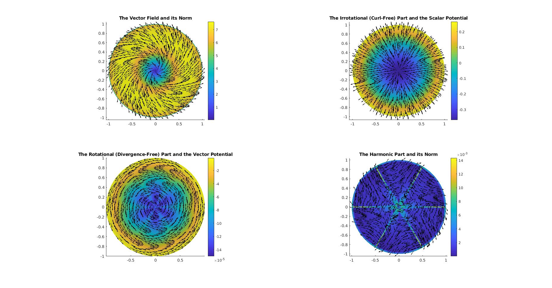
%% Perform Decomposition ==================================================
clc;
% Perform Helmholtz-Hodge decomposition
[divU, rotU, harmU, scalarP, vectorP] = ...
DEC.helmholtzHodgeDecomposition(U);
% Normalize rows for plotting
plotU = normalizerow(U);
plotDivU = normalizerow(divU);
plotRotU = normalizerow(rotU);
plotHU = normalizerow(harmU);
% Sub-sampling factor for vector field visualization
ssf = 15;
figure('Position', [0 0 800 600], 'Units', 'pixels')
% The full vector field ---------------------------------------------------
UColors = sparse( F(:), repmat(1:size(F,1),1,3), ...
internalangles(V,F), size(V,1), size(F,1) );
UColors = UColors * U;
UColors = sqrt(sum(UColors.^2, 2));
subplot(2,2,1);
patch( 'Faces', F, 'Vertices', V, 'FaceVertexCData', UColors, ...
'FaceColor', 'interp', 'EdgeColor', 'none', ...
'SpecularStrength', 0.1, 'DiffuseStrength', 0.1, ...
'AmbientStrength', 0.8 );
hold on
quiver3( COM(1:ssf:end, 1), COM(1:ssf:end, 2), COM(1:ssf:end, 3), ...
plotU(1:ssf:end, 1), plotU(1:ssf:end, 2), plotU(1:ssf:end, 3), ...
1, 'LineWidth', 2, 'Color', 'k' );
hold off
axis equal tight
camlight
title('The Vector Field and its Norm');
colorbar
% The curl-free part ------------------------------------------------------
subplot(2,2,2);
patch( 'Faces', F, 'Vertices', V, 'FaceVertexCData', scalarP, ...
'FaceColor', 'interp', 'EdgeColor', 'none', ...
'SpecularStrength', 0.1, 'DiffuseStrength', 0.1, ...
'AmbientStrength', 0.8 );
hold on
quiver3( COM(1:ssf:end, 1), COM(1:ssf:end, 2), COM(1:ssf:end, 3), ...
plotDivU(1:ssf:end, 1), plotDivU(1:ssf:end, 2), plotDivU(1:ssf:end, 3), ...
1, 'LineWidth', 2, 'Color', 'k' );
hold off
axis equal tight
camlight
title('The Irrotational (Curl-Free) Part and the Scalar Potential');
colorbar
% The divergence-free part ------------------------------------------------
subplot(2,2,3);
patch( 'Faces', F, 'Vertices', V, 'FaceVertexCData', vectorP, ...
'FaceColor', 'flat', 'EdgeColor', 'none', ...
'SpecularStrength', 0.1, 'DiffuseStrength', 0.1, ...
'AmbientStrength', 0.8 );
hold on
quiver3( COM(1:ssf:end, 1), COM(1:ssf:end, 2), COM(1:ssf:end, 3), ...
plotRotU(1:ssf:end, 1), plotRotU(1:ssf:end, 2), plotRotU(1:ssf:end, 3), ...
1, 'LineWidth', 2, 'Color', 'k' );
hold off
axis equal tight
camlight
title('The Rotational (Divergence-Free) Part and the Vector Potential');
colorbar
% The harmonic part -------------------------------------------------------
HUColors = sparse( F(:), repmat(1:size(F,1),1,3), ...
internalangles(V,F), size(V,1), size(F,1) );
HUColors = HUColors * harmU;
HUColors = sqrt(sum(HUColors.^2, 2));
subplot(2,2,4);
patch( 'Faces', F, 'Vertices', V, 'FaceVertexCData', HUColors, ...
'FaceColor', 'interp', 'EdgeColor', 'none', ...
'SpecularStrength', 0.1, 'DiffuseStrength', 0.1, ...
'AmbientStrength', 0.8 );
hold on
quiver3( COM(1:ssf:end, 1), COM(1:ssf:end, 2), COM(1:ssf:end, 3), ...
plotHU(1:ssf:end, 1), plotHU(1:ssf:end, 2), plotHU(1:ssf:end, 3), ...
1, 'LineWidth', 2, 'Color', 'k' );
hold off
axis equal tight
camlight
title('The Harmonic Part and its Norm');
colorbar
saveas(gcf, fullfile('Tutorials', ...
'DEC_sphericalMesh_decomposition.png'))
% clear ssf UColors HUColors plotU plotDivU plotRotU plotHU
%% CALCULATE ANALYIC RESULTS ==============================================
% NOTE: This section is only usable with the single supplied vector field.
% In principle one could solve the linear equations for the potentials
% analytically for an arbitrary vector field.
%
% The scalar and vector potentials are each only unique up to a pair of
% constants - their choice is arbitrary and can be absorbed into the
% harmonic component of the vector field. The discrete solution process
% will choose an unknown pair of constants to specify the potentials. In
% order to compare the solutions to analytic results we fit the constants
% to the numerical results in the least-squares sense
% Some useful parameters
cosTheta = V(:,3);
sinTheta = sin(acos(cosTheta));
tanTheta2 = tan( acos(cosTheta) ./ 2 );
cosTheta_F = mean( cosTheta(F), 2 );
sinTheta_F = mean( sinTheta(F), 2 );
tanTheta2_F = mean( tanTheta2(F), 2 );
% Generate the scalar potential -------------------------------------------
b1 = log( (1-cosTheta) ./ (1+cosTheta) ) ./ 2;
A = [ ones(size(V,1), 1), b1 ];
b = scalarP - b1 ./ 4;
Cscalar = A \ b;
trueScalarP = Cscalar(1) + Cscalar(2) .* b1 + b1 ./ 4;
% Generate the vector potential -------------------------------------------
b1 = -cosTheta_F .* sinTheta_F - log( tanTheta2_F ) ./ 2;
A = sinTheta_F .* [ log(tanTheta2_F), ones(size(F,1), 1) ];
b = vectorP - b1;
Cvector = A \b;
trueVectorP = sinTheta_F .* ( Cvector(2) + ...
Cvector(1) .* log(tanTheta2_F) ) + b1;